4.7. Pairwise metrics, Affinities and Kernels¶

The sklearn.metrics.pairwise submodule implements utilities to evaluate pairwise distances or affinity of sets of samples.

This module contains both distance metrics and kernels. A brief summary is given on the two here.

Distance metrics are functions d(a, b) such that d(a, b) < d(a, c) if objects a and b are considered “more similar” than objects a and c. Two objects exactly alike would have a distance of zero. One of the most popular examples is Euclidean distance. To be a ‘true’ metric, it must obey the following four conditions:

d(a, b) >= 0, for all a and b
d(a, b) == 0, if and only if a = b, positive definiteness
d(a, b) == d(b, a), symmetry
d(a, c) <= d(a, b) + d(b, c), the triangle inequality

Kernels are measures of similarity, i.e. s(a, b) > s(a, c) if objects a and b are considered “more similar” than objects a and c. A kernel must also be positive semi-definite.

There are a number of ways to convert between a distance metric and a similarity measure, such as a kernel. Let D be the distance, and S be the kernel:

S = np.exp(-D * gamma), where one heuristic for choosing gamma is 1 / num_features

S = 1. / (D / np.max(D))

4.7.1. Cosine similarity¶

cosine_similarity computes the L2-normalized dot product of vectors. That is, if $x$ and $y$ are row vectors, their cosine similarity $k$ is defined as:

$k(x, y) = \frac{x y^\top}{\|x\| \|y\|}$

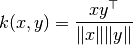
This is called cosine similarity, because Euclidean (L2) normalization projects the vectors onto the unit sphere, and their dot product is then the cosine of the angle between the points denoted by the vectors.

This kernel is a popular choice for computing the similarity of documents represented as tf-idf vectors. cosine_similarity accepts scipy.sparse matrices. (Note that the tf-idf functionality in sklearn.feature_extraction.text can produce normalized vectors, in which case cosine_similarity is equivalent to linear_kernel, only slower.)

References:

C.D. Manning, P. Raghavan and H. Schütze (2008). Introduction to Information Retrieval. Cambridge University Press. http://nlp.stanford.edu/IR-book/html/htmledition/the-vector-space-model-for-scoring-1.html

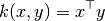
4.7.2. Linear kernel¶

The function linear_kernel computes the linear kernel, that is, a special case of polynomial_kernel with degree=1 and coef0=0 (homogeneous). If x and y are column vectors, their linear kernel is:

$k(x, y) = x^\top y$

4.7.3. Polynomial kernel¶

The function polynomial_kernel computes the degree-d polynomial kernel between two vectors. The polynomial kernel represents the similarity between two vectors. Conceptually, the polynomial kernels considers not only the similarity between vectors under the same dimension, but also across dimensions. When used in machine learning algorithms, this allows to account for feature interaction.

The polynomial kernel is defined as:

$k(x, y) = (\gamma x^\top y +c_0)^d$

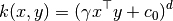
where:

x, y are the input vectors

d is the kernel degree

If $c_0 = 0$ the kernel is said to be homogeneous.

4.7.4. Sigmoid kernel¶

The function sigmoid_kernel computes the sigmoid kernel between two vectors. The sigmoid kernel is also known as hyperbolic tangent, or Multilayer Perceptron (because, in the neural network field, it is often used as neuron activation function). It is defined as:

$k(x, y) = \tanh( \gamma x^\top y + c_0)$

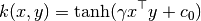
where:

x, y are the input vectors

$\gamma$ is known as slope

$c_0$ is known as intercept

4.7.5. RBF kernel¶

The function rbf_kernel computes the radial basis function (RBF) kernel between two vectors. This kernel is defined as:

$k(x, y) = \exp( -\gamma \| x-y \|^2)$

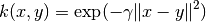
where x and y are the input vectors. If $\gamma = \sigma^{-2}$ the kernel is known as the Gaussian kernel of variance $\sigma^2$ .

4.7.6. Chi-squared kernel¶

The chi-squared kernel is a very popular choice for training non-linear SVMs in computer vision applications. It can be computed using chi2_kernel and then passed to an sklearn.svm.SVC with kernel="precomputed":

>>> from sklearn.svm import SVC
>>> from sklearn.metrics.pairwise import chi2_kernel
>>> X = [[0, 1], [1, 0], [.2, .8], [.7, .3]]
>>> y = [0, 1, 0, 1]
>>> K = chi2_kernel(X, gamma=.5)
>>> K                        
array([[ 1.        ,  0.36...,  0.89...,  0.58...],
       [ 0.36...,  1.        ,  0.51...,  0.83...],
       [ 0.89...,  0.51...,  1.        ,  0.77... ],
       [ 0.58...,  0.83...,  0.77... ,  1.        ]])

>>> svm = SVC(kernel='precomputed').fit(K, y)
>>> svm.predict(K)
array([0, 1, 0, 1])

It can also be directly used as the kernel argument:

>>> svm = SVC(kernel=chi2_kernel).fit(X, y)
>>> svm.predict(X)
array([0, 1, 0, 1])

The chi squared kernel is given by

$k(x, y) = \exp \left (-\gamma \sum_i \frac{(x[i] - y[i]) ^ 2}{x[i] + y[i]} \right )$

The data is assumed to be non-negative, and is often normalized to have an L1-norm of one. The normalization is rationalized with the connection to the chi squared distance, which is a distance between discrete probability distributions.

The chi squared kernel is most commonly used on histograms (bags) of visual words.

References:

Zhang, J. and Marszalek, M. and Lazebnik, S. and Schmid, C. Local features and kernels for classification of texture and object categories: A comprehensive study International Journal of Computer Vision 2007 http://eprints.pascal-network.org/archive/00002309/01/Zhang06-IJCV.pdf