Gaussian Mixture Model Sine Curve

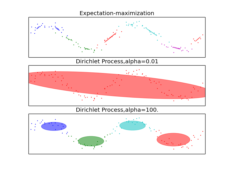
This example highlights the advantages of the Dirichlet Process: complexity control and dealing with sparse data. The dataset is formed by 100 points loosely spaced following a noisy sine curve. The fit by the GMM class, using the expectation-maximization algorithm to fit a mixture of 10 Gaussian components, finds too-small components and very little structure. The fits by the Dirichlet process, however, show that the model can either learn a global structure for the data (small alpha) or easily interpolate to finding relevant local structure (large alpha), never falling into the problems shown by the GMM class.

Python source code: plot_gmm_sin.py

import itertools

import numpy as np
from scipy import linalg
import matplotlib.pyplot as plt
import matplotlib as mpl

from sklearn import mixture
from sklearn.externals.six.moves import xrange

# Number of samples per component
n_samples = 100

# Generate random sample following a sine curve
np.random.seed(0)
X = np.zeros((n_samples, 2))
step = 4 * np.pi / n_samples

for i in xrange(X.shape[0]):
    x = i * step - 6
    X[i, 0] = x + np.random.normal(0, 0.1)
    X[i, 1] = 3 * (np.sin(x) + np.random.normal(0, .2))


color_iter = itertools.cycle(['r', 'g', 'b', 'c', 'm'])


for i, (clf, title) in enumerate([
        (mixture.GMM(n_components=10, covariance_type='full', n_iter=100),
         "Expectation-maximization"),
        (mixture.DPGMM(n_components=10, covariance_type='full', alpha=0.01,
                       n_iter=100),
         "Dirichlet Process,alpha=0.01"),
        (mixture.DPGMM(n_components=10, covariance_type='diag', alpha=100.,
                       n_iter=100),
         "Dirichlet Process,alpha=100.")]):

    clf.fit(X)
    splot = plt.subplot(3, 1, 1 + i)
    Y_ = clf.predict(X)
    for i, (mean, covar, color) in enumerate(zip(
            clf.means_, clf._get_covars(), color_iter)):
        v, w = linalg.eigh(covar)
        u = w[0] / linalg.norm(w[0])
        # as the DP will not use every component it has access to
        # unless it needs it, we shouldn't plot the redundant
        # components.
        if not np.any(Y_ == i):
            continue
        plt.scatter(X[Y_ == i, 0], X[Y_ == i, 1], .8, color=color)

        # Plot an ellipse to show the Gaussian component
        angle = np.arctan(u[1] / u[0])
        angle = 180 * angle / np.pi  # convert to degrees
        ell = mpl.patches.Ellipse(mean, v[0], v[1], 180 + angle, color=color)
        ell.set_clip_box(splot.bbox)
        ell.set_alpha(0.5)
        splot.add_artist(ell)

    plt.xlim(-6, 4 * np.pi - 6)
    plt.ylim(-5, 5)
    plt.title(title)
    plt.xticks(())
    plt.yticks(())

plt.show()

Total running time of the example: 0.44 seconds ( 0 minutes 0.44 seconds)