
1.13. Feature selection
The classes in the sklearn.feature_selection module can be used
for feature selection/dimensionality reduction on sample sets, either to
improve estimators’ accuracy scores or to boost their performance on very
high-dimensional datasets.
1.13.1. Removing features with low variance
VarianceThreshold is a simple baseline approach to feature selection.
It removes all features whose variance doesn’t meet some threshold.
By default, it removes all zero-variance features,
i.e. features that have the same value in all samples.
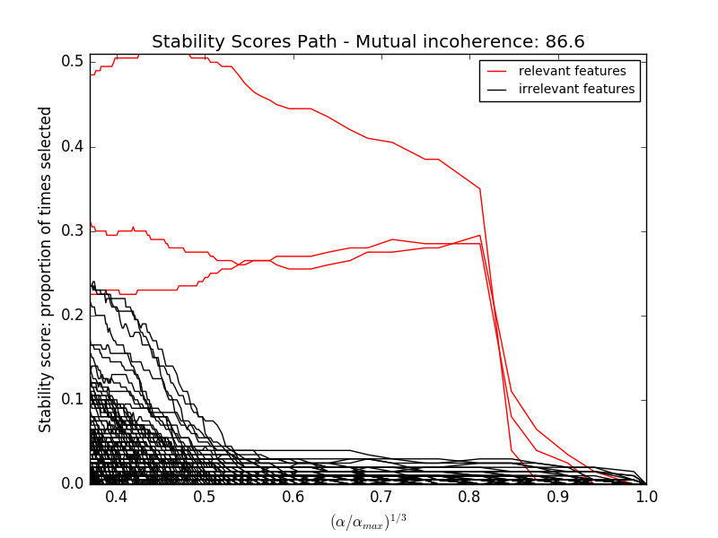
As an example, suppose that we have a dataset with boolean features, and we want to remove all features that are either one or zero (on or off) in more than 80% of the samples. Boolean features are Bernoulli random variables, and the variance of such variables is given by
![\mathrm{Var}[X] = p(1 - p)](../_images/math/415d9594608f0ddd0c80635c2fcce650e402d81b.png)
so we can select using the threshold .8 * (1 - .8):
>>> from sklearn.feature_selection import VarianceThreshold
>>> X = [[0, 0, 1], [0, 1, 0], [1, 0, 0], [0, 1, 1], [0, 1, 0], [0, 1, 1]]
>>> sel = VarianceThreshold(threshold=(.8 * (1 - .8)))
>>> sel.fit_transform(X)
array([[0, 1],
       [1, 0],
       [0, 0],
       [1, 1],
       [1, 0],
       [1, 1]])
As expected, VarianceThreshold has removed the first column,
which has a probability  of containing a zero.
1.13.2. Univariate feature selection
Univariate feature selection works by selecting the best features based on
univariate statistical tests. It can be seen as a preprocessing step
to an estimator. Scikit-learn exposes feature selection routines
as objects that implement the transform method:
SelectKBestremoves all but thehighest scoring features
SelectPercentileremoves all but a user-specified highest scoring percentage of features- using common univariate statistical tests for each feature: false positive rate
SelectFpr, false discovery rateSelectFdr, or family wise errorSelectFwe.GenericUnivariateSelectallows to perform univariate feature selection with a configurable strategy. This allows to select the best univariate selection strategy with hyper-parameter search estimator.
For instance, we can perform a  test to the samples
to retrieve only the two best features as follows:
test to the samples
to retrieve only the two best features as follows:
>>> from sklearn.datasets import load_iris
>>> from sklearn.feature_selection import SelectKBest
>>> from sklearn.feature_selection import chi2
>>> iris = load_iris()
>>> X, y = iris.data, iris.target
>>> X.shape
(150, 4)
>>> X_new = SelectKBest(chi2, k=2).fit_transform(X, y)
>>> X_new.shape
(150, 2)
These objects take as input a scoring function that returns univariate scores
and p-values (or only scores for SelectKBest and
SelectPercentile):
- For regression:
f_regression,mutual_info_regression- For classification:
chi2,f_classif,mutual_info_classif
The methods based on F-test estimate the degree of linear dependency between two random variables. On the other hand, mutual information methods can capture any kind of statistical dependency, but being nonparametric, they require more samples for accurate estimation.
Feature selection with sparse data
If you use sparse data (i.e. data represented as sparse matrices),
chi2, mutual_info_regression, mutual_info_classif
will deal with the data without making it dense.
Warning
Beware not to use a regression scoring function with a classification problem, you will get useless results.
1.13.3. Recursive feature elimination
Given an external estimator that assigns weights to features (e.g., the
coefficients of a linear model), recursive feature elimination (RFE)
is to select features by recursively considering smaller and smaller sets of
features. First, the estimator is trained on the initial set of features and
weights are assigned to each one of them. Then, features whose absolute weights
are the smallest are pruned from the current set features. That procedure is
recursively repeated on the pruned set until the desired number of features to
select is eventually reached.
RFECV performs RFE in a cross-validation loop to find the optimal
number of features.
Examples:
- Recursive feature elimination: A recursive feature elimination example showing the relevance of pixels in a digit classification task.
- Recursive feature elimination with cross-validation: A recursive feature elimination example with automatic tuning of the number of features selected with cross-validation.
1.13.4. Feature selection using SelectFromModel
SelectFromModel is a meta-transformer that can be used along with any
estimator that has a coef_ or feature_importances_ attribute after fitting.
The features are considered unimportant and removed, if the corresponding
coef_ or feature_importances_ values are below the provided
threshold parameter. Apart from specifying the threshold numerically,
there are built-in heuristics for finding a threshold using a string argument.
Available heuristics are “mean”, “median” and float multiples of these like
“0.1*mean”.
For examples on how it is to be used refer to the sections below.
Examples
- Feature selection using SelectFromModel and LassoCV: Selecting the two most important features from the Boston dataset without knowing the threshold beforehand.
1.13.4.1. L1-based feature selection
Linear models penalized with the L1 norm have
sparse solutions: many of their estimated coefficients are zero. When the goal
is to reduce the dimensionality of the data to use with another classifier,
they can be used along with feature_selection.SelectFromModel
to select the non-zero coefficients. In particular, sparse estimators useful
for this purpose are the linear_model.Lasso for regression, and
of linear_model.LogisticRegression and svm.LinearSVC
for classification:
>>> from sklearn.svm import LinearSVC
>>> from sklearn.datasets import load_iris
>>> from sklearn.feature_selection import SelectFromModel
>>> iris = load_iris()
>>> X, y = iris.data, iris.target
>>> X.shape
(150, 4)
>>> lsvc = LinearSVC(C=0.01, penalty="l1", dual=False).fit(X, y)
>>> model = SelectFromModel(lsvc, prefit=True)
>>> X_new = model.transform(X)
>>> X_new.shape
(150, 3)
With SVMs and logistic-regression, the parameter C controls the sparsity: the smaller C the fewer features selected. With Lasso, the higher the alpha parameter, the fewer features selected.
Examples:
- Classification of text documents using sparse features: Comparison of different algorithms for document classification including L1-based feature selection.
L1-recovery and compressive sensing
For a good choice of alpha, the Lasso can fully recover the exact set of non-zero variables using only few observations, provided certain specific conditions are met. In particular, the number of samples should be “sufficiently large”, or L1 models will perform at random, where “sufficiently large” depends on the number of non-zero coefficients, the logarithm of the number of features, the amount of noise, the smallest absolute value of non-zero coefficients, and the structure of the design matrix X. In addition, the design matrix must display certain specific properties, such as not being too correlated.
There is no general rule to select an alpha parameter for recovery of
non-zero coefficients. It can by set by cross-validation
(LassoCV or LassoLarsCV), though this may lead to
under-penalized models: including a small number of non-relevant
variables is not detrimental to prediction score. BIC
(LassoLarsIC) tends, on the opposite, to set high values of
alpha.
Reference Richard G. Baraniuk “Compressive Sensing”, IEEE Signal Processing Magazine [120] July 2007 http://dsp.rice.edu/sites/dsp.rice.edu/files/cs/baraniukCSlecture07.pdf
1.13.4.2. Randomized sparse models
In terms of feature selection, there are some well-known limitations of L1-penalized models for regression and classification. For example, it is known that the Lasso will tend to select an individual variable out of a group of highly correlated features. Furthermore, even when the correlation between features is not too high, the conditions under which L1-penalized methods consistently select “good” features can be restrictive in general.
To mitigate this problem, it is possible to use randomization techniques such
as those presented in [B2009] and [M2010]. The latter technique, known as
stability selection, is implemented in the module sklearn.linear_model.
In the stability selection method, a subsample of the data is fit to a
L1-penalized model where the penalty of a random subset of coefficients has
been scaled. Specifically, given a subsample of the data
 , where
 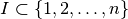 is a
random subset of the data of size
is a
random subset of the data of size  , the following modified Lasso
fit is obtained:
, the following modified Lasso
fit is obtained:
where  are independent trials of a fair Bernoulli
random variable, and
are independent trials of a fair Bernoulli
random variable, and  is the scaling factor. By repeating this
procedure across different random subsamples and Bernoulli trials, one can
count the fraction of times the randomized procedure selected each feature,
and used these fractions as scores for feature selection.
is the scaling factor. By repeating this
procedure across different random subsamples and Bernoulli trials, one can
count the fraction of times the randomized procedure selected each feature,
and used these fractions as scores for feature selection.
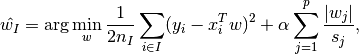
RandomizedLasso implements this strategy for regression
settings, using the Lasso, while RandomizedLogisticRegression uses the
logistic regression and is suitable for classification tasks. To get a full
path of stability scores you can use lasso_stability_path.
Note that for randomized sparse models to be more powerful than standard F statistics at detecting non-zero features, the ground truth model should be sparse, in other words, there should be only a small fraction of features non zero.
Examples:
- Sparse recovery: feature selection for sparse linear models: An example comparing different feature selection approaches and discussing in which situation each approach is to be favored.
References:
| [B2009] | F. Bach, “Model-Consistent Sparse Estimation through the Bootstrap.” https://hal.inria.fr/hal-00354771/ |
| [M2010] | N. Meinshausen, P. Buhlmann, “Stability selection”, Journal of the Royal Statistical Society, 72 (2010) http://arxiv.org/pdf/0809.2932.pdf |
1.13.4.3. Tree-based feature selection
Tree-based estimators (see the sklearn.tree module and forest
of trees in the sklearn.ensemble module) can be used to compute
feature importances, which in turn can be used to discard irrelevant
features (when coupled with the sklearn.feature_selection.SelectFromModel
meta-transformer):
>>> from sklearn.ensemble import ExtraTreesClassifier
>>> from sklearn.datasets import load_iris
>>> from sklearn.feature_selection import SelectFromModel
>>> iris = load_iris()
>>> X, y = iris.data, iris.target
>>> X.shape
(150, 4)
>>> clf = ExtraTreesClassifier()
>>> clf = clf.fit(X, y)
>>> clf.feature_importances_
array([ 0.04...,  0.05...,  0.4...,  0.4...])
>>> model = SelectFromModel(clf, prefit=True)
>>> X_new = model.transform(X)
>>> X_new.shape
(150, 2)
Examples:
- Feature importances with forests of trees: example on synthetic data showing the recovery of the actually meaningful features.
- Pixel importances with a parallel forest of trees: example on face recognition data.
1.13.5. Feature selection as part of a pipeline
Feature selection is usually used as a pre-processing step before doing
the actual learning. The recommended way to do this in scikit-learn is
to use a sklearn.pipeline.Pipeline:
clf = Pipeline([
  ('feature_selection', SelectFromModel(LinearSVC(penalty="l1"))),
  ('classification', RandomForestClassifier())
])
clf.fit(X, y)
In this snippet we make use of a sklearn.svm.LinearSVC
coupled with sklearn.feature_selection.SelectFromModel
to evaluate feature importances and select the most relevant features.
Then, a sklearn.ensemble.RandomForestClassifier is trained on the
transformed output, i.e. using only relevant features. You can perform
similar operations with the other feature selection methods and also
classifiers that provide a way to evaluate feature importances of course.
See the sklearn.pipeline.Pipeline examples for more details.