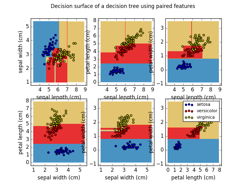
Plot the decision surface of a decision tree on the iris dataset

Plot the decision surface of a decision tree trained on pairs of features of the iris dataset.

See decision tree for more information on the estimator.

For each pair of iris features, the decision tree learns decision boundaries made of combinations of simple thresholding rules inferred from the training samples.

print(__doc__)

import numpy as np
import matplotlib.pyplot as plt

from sklearn.datasets import load_iris
from sklearn.tree import DecisionTreeClassifier

# Parameters
n_classes = 3
plot_colors = "bry"
plot_step = 0.02

# Load data
iris = load_iris()

for pairidx, pair in enumerate([[0, 1], [0, 2], [0, 3],
                                [1, 2], [1, 3], [2, 3]]):
    # We only take the two corresponding features
    X = iris.data[:, pair]
    y = iris.target

    # Train
    clf = DecisionTreeClassifier().fit(X, y)

    # Plot the decision boundary
    plt.subplot(2, 3, pairidx + 1)

    x_min, x_max = X[:, 0].min() - 1, X[:, 0].max() + 1
    y_min, y_max = X[:, 1].min() - 1, X[:, 1].max() + 1
    xx, yy = np.meshgrid(np.arange(x_min, x_max, plot_step),
                         np.arange(y_min, y_max, plot_step))

    Z = clf.predict(np.c_[xx.ravel(), yy.ravel()])
    Z = Z.reshape(xx.shape)
    cs = plt.contourf(xx, yy, Z, cmap=plt.cm.Paired)

    plt.xlabel(iris.feature_names[pair[0]])
    plt.ylabel(iris.feature_names[pair[1]])
    plt.axis("tight")

    # Plot the training points
    for i, color in zip(range(n_classes), plot_colors):
        idx = np.where(y == i)
        plt.scatter(X[idx, 0], X[idx, 1], c=color, label=iris.target_names[i],
                    cmap=plt.cm.Paired)

    plt.axis("tight")

plt.suptitle("Decision surface of a decision tree using paired features")
plt.legend()
plt.show()

Total running time of the script: (0 minutes 0.514 seconds)

Download Python source code: plot_iris.py

Download IPython notebook: plot_iris.ipynb