Sparsity Example: Fitting only features 1 and 2

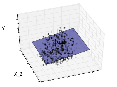
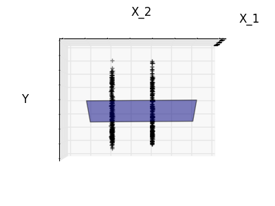
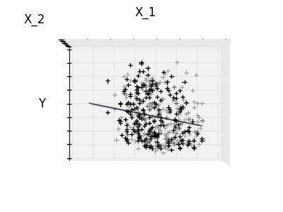
Features 1 and 2 of the diabetes-dataset are fitted and plotted below. It illustrates that although feature 2 has a strong coefficient on the full model, it does not give us much regarding y when compared to just feature 1

print(__doc__)


# Code source: Gaël Varoquaux
# Modified for documentation by Jaques Grobler
# License: BSD 3 clause

import matplotlib.pyplot as plt
import numpy as np
from mpl_toolkits.mplot3d import Axes3D

from sklearn import datasets, linear_model

diabetes = datasets.load_diabetes()
indices = (0, 1)

X_train = diabetes.data[:-20, indices]
X_test = diabetes.data[-20:, indices]
y_train = diabetes.target[:-20]
y_test = diabetes.target[-20:]

ols = linear_model.LinearRegression()
ols.fit(X_train, y_train)

Plot the figure

def plot_figs(fig_num, elev, azim, X_train, clf):
    fig = plt.figure(fig_num, figsize=(4, 3))
    plt.clf()
    ax = Axes3D(fig, elev=elev, azim=azim)

    ax.scatter(X_train[:, 0], X_train[:, 1], y_train, c='k', marker='+')
    ax.plot_surface(np.array([[-.1, -.1], [.15, .15]]),
                    np.array([[-.1, .15], [-.1, .15]]),
                    clf.predict(np.array([[-.1, -.1, .15, .15],
                                          [-.1, .15, -.1, .15]]).T
                                ).reshape((2, 2)),
                    alpha=.5)
    ax.set_xlabel('X_1')
    ax.set_ylabel('X_2')
    ax.set_zlabel('Y')
    ax.w_xaxis.set_ticklabels([])
    ax.w_yaxis.set_ticklabels([])
    ax.w_zaxis.set_ticklabels([])

#Generate the three different figures from different views
elev = 43.5
azim = -110
plot_figs(1, elev, azim, X_train, ols)

elev = -.5
azim = 0
plot_figs(2, elev, azim, X_train, ols)

elev = -.5
azim = 90
plot_figs(3, elev, azim, X_train, ols)

plt.show()

• 
• 
• 

Total running time of the script: (0 minutes 0.329 seconds)

Download Python source code: plot_ols_3d.py

Download IPython notebook: plot_ols_3d.ipynb