Bayesian Ridge Regression¶

Computes a Bayesian Ridge Regression on a synthetic dataset.

See Bayesian Ridge Regression for more information on the regressor.

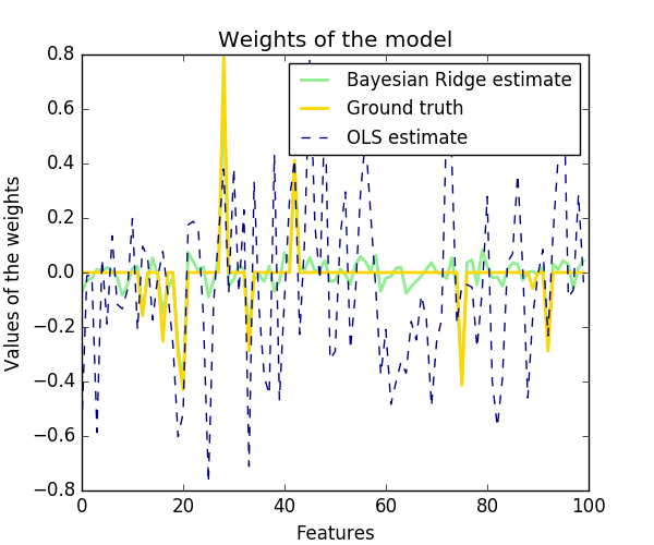
Compared to the OLS (ordinary least squares) estimator, the coefficient weights are slightly shifted toward zeros, which stabilises them.

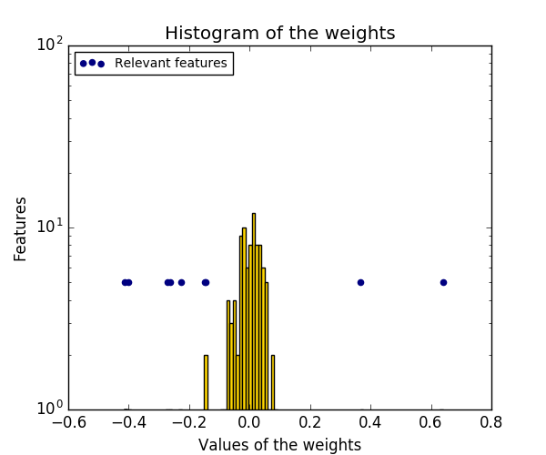
As the prior on the weights is a Gaussian prior, the histogram of the estimated weights is Gaussian.

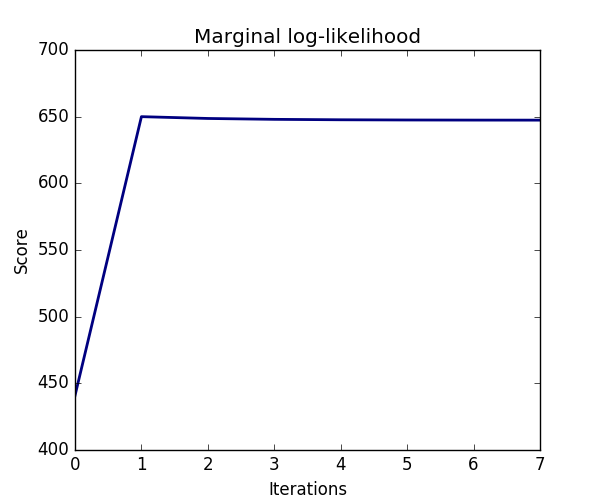
The estimation of the model is done by iteratively maximizing the marginal log-likelihood of the observations.

print(__doc__)

import numpy as np
import matplotlib.pyplot as plt
from scipy import stats

from sklearn.linear_model import BayesianRidge, LinearRegression

Generating simulated data with Gaussian weights

np.random.seed(0)
n_samples, n_features = 100, 100
X = np.random.randn(n_samples, n_features)  # Create Gaussian data
# Create weights with a precision lambda_ of 4.
lambda_ = 4.
w = np.zeros(n_features)
# Only keep 10 weights of interest
relevant_features = np.random.randint(0, n_features, 10)
for i in relevant_features:
    w[i] = stats.norm.rvs(loc=0, scale=1. / np.sqrt(lambda_))
# Create noise with a precision alpha of 50.
alpha_ = 50.
noise = stats.norm.rvs(loc=0, scale=1. / np.sqrt(alpha_), size=n_samples)
# Create the target
y = np.dot(X, w) + noise

Fit the Bayesian Ridge Regression and an OLS for comparison

clf = BayesianRidge(compute_score=True)
clf.fit(X, y)

ols = LinearRegression()
ols.fit(X, y)

Plot true weights, estimated weights and histogram of the weights

lw = 2
plt.figure(figsize=(6, 5))
plt.title("Weights of the model")
plt.plot(clf.coef_, color='lightgreen', linewidth=lw,
         label="Bayesian Ridge estimate")
plt.plot(w, color='gold', linewidth=lw, label="Ground truth")
plt.plot(ols.coef_, color='navy', linestyle='--', label="OLS estimate")
plt.xlabel("Features")
plt.ylabel("Values of the weights")
plt.legend(loc="best", prop=dict(size=12))

plt.figure(figsize=(6, 5))
plt.title("Histogram of the weights")
plt.hist(clf.coef_, bins=n_features, color='gold', log=True)
plt.scatter(clf.coef_[relevant_features], 5 * np.ones(len(relevant_features)),
            color='navy', label="Relevant features")
plt.ylabel("Features")
plt.xlabel("Values of the weights")
plt.legend(loc="upper left")

plt.figure(figsize=(6, 5))
plt.title("Marginal log-likelihood")
plt.plot(clf.scores_, color='navy', linewidth=lw)
plt.ylabel("Score")
plt.xlabel("Iterations")
plt.show()

Total running time of the script: (0 minutes 0.345 seconds)

Download Python source code: plot_bayesian_ridge.py

Download IPython notebook: plot_bayesian_ridge.ipynb