
Gaussian process regression (GPR) with noise-level estimation
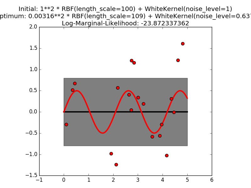
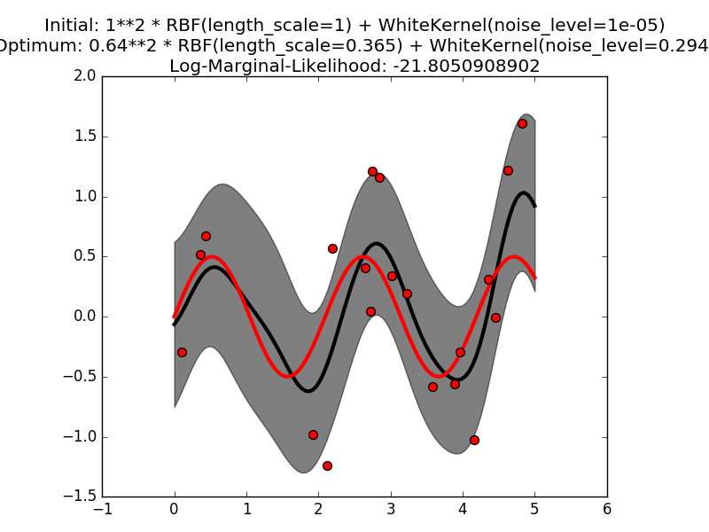
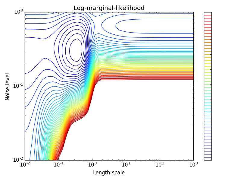
This example illustrates that GPR with a sum-kernel including a WhiteKernel can estimate the noise level of data. An illustration of the log-marginal-likelihood (LML) landscape shows that there exist two local maxima of LML. The first corresponds to a model with a high noise level and a large length scale, which explains all variations in the data by noise. The second one has a smaller noise level and shorter length scale, which explains most of the variation by the noise-free functional relationship. The second model has a higher likelihood; however, depending on the initial value for the hyperparameters, the gradient-based optimization might also converge to the high-noise solution. It is thus important to repeat the optimization several times for different initializations.
print(__doc__)

# Authors: Jan Hendrik Metzen <jhm@informatik.uni-bremen.de>
#
# License: BSD 3 clause

import numpy as np

from matplotlib import pyplot as plt
from matplotlib.colors import LogNorm

from sklearn.gaussian_process import GaussianProcessRegressor
from sklearn.gaussian_process.kernels import RBF, WhiteKernel


rng = np.random.RandomState(0)
X = rng.uniform(0, 5, 20)[:, np.newaxis]
y = 0.5 * np.sin(3 * X[:, 0]) + rng.normal(0, 0.5, X.shape[0])

# First run
plt.figure(0)
kernel = 1.0 * RBF(length_scale=100.0, length_scale_bounds=(1e-2, 1e3)) \
    + WhiteKernel(noise_level=1, noise_level_bounds=(1e-10, 1e+1))
gp = GaussianProcessRegressor(kernel=kernel,
                              alpha=0.0).fit(X, y)
X_ = np.linspace(0, 5, 100)
y_mean, y_cov = gp.predict(X_[:, np.newaxis], return_cov=True)
plt.plot(X_, y_mean, 'k', lw=3, zorder=9)
plt.fill_between(X_, y_mean - np.sqrt(np.diag(y_cov)),
                 y_mean + np.sqrt(np.diag(y_cov)),
                 alpha=0.5, color='k')
plt.plot(X_, 0.5*np.sin(3*X_), 'r', lw=3, zorder=9)
plt.scatter(X[:, 0], y, c='r', s=50, zorder=10)
plt.title("Initial: %s\nOptimum: %s\nLog-Marginal-Likelihood: %s"
          % (kernel, gp.kernel_,
             gp.log_marginal_likelihood(gp.kernel_.theta)))
plt.tight_layout()

# Second run
plt.figure(1)
kernel = 1.0 * RBF(length_scale=1.0, length_scale_bounds=(1e-2, 1e3)) \
    + WhiteKernel(noise_level=1e-5, noise_level_bounds=(1e-10, 1e+1))
gp = GaussianProcessRegressor(kernel=kernel,
                              alpha=0.0).fit(X, y)
X_ = np.linspace(0, 5, 100)
y_mean, y_cov = gp.predict(X_[:, np.newaxis], return_cov=True)
plt.plot(X_, y_mean, 'k', lw=3, zorder=9)
plt.fill_between(X_, y_mean - np.sqrt(np.diag(y_cov)),
                 y_mean + np.sqrt(np.diag(y_cov)),
                 alpha=0.5, color='k')
plt.plot(X_, 0.5*np.sin(3*X_), 'r', lw=3, zorder=9)
plt.scatter(X[:, 0], y, c='r', s=50, zorder=10)
plt.title("Initial: %s\nOptimum: %s\nLog-Marginal-Likelihood: %s"
          % (kernel, gp.kernel_,
             gp.log_marginal_likelihood(gp.kernel_.theta)))
plt.tight_layout()

# Plot LML landscape
plt.figure(2)
theta0 = np.logspace(-2, 3, 49)
theta1 = np.logspace(-2, 0, 50)
Theta0, Theta1 = np.meshgrid(theta0, theta1)
LML = [[gp.log_marginal_likelihood(np.log([0.36, Theta0[i, j], Theta1[i, j]]))
        for i in range(Theta0.shape[0])] for j in range(Theta0.shape[1])]
LML = np.array(LML).T

vmin, vmax = (-LML).min(), (-LML).max()
vmax = 50
plt.contour(Theta0, Theta1, -LML,
            levels=np.logspace(np.log10(vmin), np.log10(vmax), 50),
            norm=LogNorm(vmin=vmin, vmax=vmax))
plt.colorbar()
plt.xscale("log")
plt.yscale("log")
plt.xlabel("Length-scale")
plt.ylabel("Noise-level")
plt.title("Log-marginal-likelihood")
plt.tight_layout()

plt.show()
Total running time of the script: (0 minutes 10.482 seconds)
plot_gpr_noisy.pyplot_gpr_noisy.ipynb