Gradient Boosting regularization

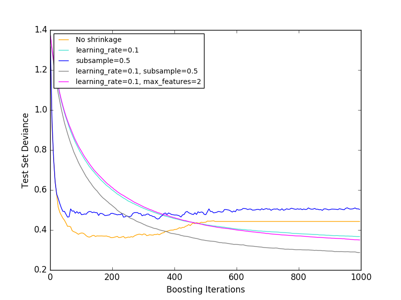
Illustration of the effect of different regularization strategies for Gradient Boosting. The example is taken from Hastie et al 2009.

The loss function used is binomial deviance. Regularization via shrinkage (learning_rate < 1.0) improves performance considerably. In combination with shrinkage, stochastic gradient boosting (subsample < 1.0) can produce more accurate models by reducing the variance via bagging. Subsampling without shrinkage usually does poorly. Another strategy to reduce the variance is by subsampling the features analogous to the random splits in Random Forests (via the max_features parameter).

[1]	T. Hastie, R. Tibshirani and J. Friedman, “Elements of Statistical Learning Ed. 2”, Springer, 2009.

print(__doc__)

# Author: Peter Prettenhofer <peter.prettenhofer@gmail.com>
#
# License: BSD 3 clause

import numpy as np
import matplotlib.pyplot as plt

from sklearn import ensemble
from sklearn import datasets


X, y = datasets.make_hastie_10_2(n_samples=12000, random_state=1)
X = X.astype(np.float32)

# map labels from {-1, 1} to {0, 1}
labels, y = np.unique(y, return_inverse=True)

X_train, X_test = X[:2000], X[2000:]
y_train, y_test = y[:2000], y[2000:]

original_params = {'n_estimators': 1000, 'max_leaf_nodes': 4, 'max_depth': None, 'random_state': 2,
                   'min_samples_split': 5}

plt.figure()

for label, color, setting in [('No shrinkage', 'orange',
                               {'learning_rate': 1.0, 'subsample': 1.0}),
                              ('learning_rate=0.1', 'turquoise',
                               {'learning_rate': 0.1, 'subsample': 1.0}),
                              ('subsample=0.5', 'blue',
                               {'learning_rate': 1.0, 'subsample': 0.5}),
                              ('learning_rate=0.1, subsample=0.5', 'gray',
                               {'learning_rate': 0.1, 'subsample': 0.5}),
                              ('learning_rate=0.1, max_features=2', 'magenta',
                               {'learning_rate': 0.1, 'max_features': 2})]:
    params = dict(original_params)
    params.update(setting)

    clf = ensemble.GradientBoostingClassifier(**params)
    clf.fit(X_train, y_train)

    # compute test set deviance
    test_deviance = np.zeros((params['n_estimators'],), dtype=np.float64)

    for i, y_pred in enumerate(clf.staged_decision_function(X_test)):
        # clf.loss_ assumes that y_test[i] in {0, 1}
        test_deviance[i] = clf.loss_(y_test, y_pred)

    plt.plot((np.arange(test_deviance.shape[0]) + 1)[::5], test_deviance[::5],
            '-', color=color, label=label)

plt.legend(loc='upper left')
plt.xlabel('Boosting Iterations')
plt.ylabel('Test Set Deviance')

plt.show()

Total running time of the script: (0 minutes 12.004 seconds)

Download Python source code: plot_gradient_boosting_regularization.py

Download IPython notebook: plot_gradient_boosting_regularization.ipynb