
Pipelining: chaining a PCA and a logistic regression
The PCA does an unsupervised dimensionality reduction, while the logistic regression does the prediction.
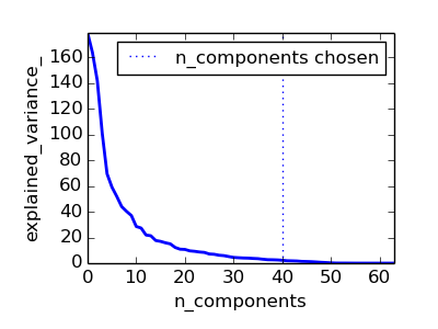
We use a GridSearchCV to set the dimensionality of the PCA
Python source code: plot_digits_pipe.py
print(__doc__)


# Code source: Gaël Varoquaux
# Modified for documentation by Jaques Grobler
# License: BSD 3 clause


import numpy as np
import matplotlib.pyplot as plt

from sklearn import linear_model, decomposition, datasets
from sklearn.pipeline import Pipeline
from sklearn.grid_search import GridSearchCV

logistic = linear_model.LogisticRegression()

pca = decomposition.PCA()
pipe = Pipeline(steps=[('pca', pca), ('logistic', logistic)])

digits = datasets.load_digits()
X_digits = digits.data
y_digits = digits.target

###############################################################################
# Plot the PCA spectrum
pca.fit(X_digits)

plt.figure(1, figsize=(4, 3))
plt.clf()
plt.axes([.2, .2, .7, .7])
plt.plot(pca.explained_variance_, linewidth=2)
plt.axis('tight')
plt.xlabel('n_components')
plt.ylabel('explained_variance_')

###############################################################################
# Prediction

n_components = [20, 40, 64]
Cs = np.logspace(-4, 4, 3)

#Parameters of pipelines can be set using ‘__’ separated parameter names:

estimator = GridSearchCV(pipe,
                         dict(pca__n_components=n_components,
                              logistic__C=Cs))
estimator.fit(X_digits, y_digits)

plt.axvline(estimator.best_estimator_.named_steps['pca'].n_components,
            linestyle=':', label='n_components chosen')
plt.legend(prop=dict(size=12))
plt.show()
Total running time of the example: 8.43 seconds ( 0 minutes 8.43 seconds)