Comparing different clustering algorithms on toy datasets

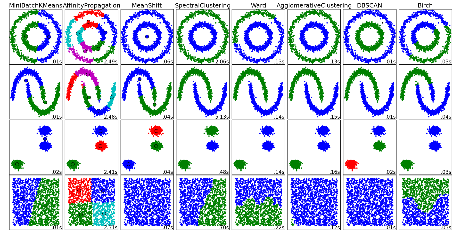
This example aims at showing characteristics of different clustering algorithms on datasets that are “interesting” but still in 2D. The last dataset is an example of a ‘null’ situation for clustering: the data is homogeneous, and there is no good clustering.

While these examples give some intuition about the algorithms, this intuition might not apply to very high dimensional data.

The results could be improved by tweaking the parameters for each clustering strategy, for instance setting the number of clusters for the methods that needs this parameter specified. Note that affinity propagation has a tendency to create many clusters. Thus in this example its two parameters (damping and per-point preference) were set to to mitigate this behavior.

Python source code: plot_cluster_comparison.py

print(__doc__)

import time

import numpy as np
import matplotlib.pyplot as plt

from sklearn import cluster, datasets
from sklearn.neighbors import kneighbors_graph
from sklearn.preprocessing import StandardScaler

np.random.seed(0)

# Generate datasets. We choose the size big enough to see the scalability
# of the algorithms, but not too big to avoid too long running times
n_samples = 1500
noisy_circles = datasets.make_circles(n_samples=n_samples, factor=.5,
                                      noise=.05)
noisy_moons = datasets.make_moons(n_samples=n_samples, noise=.05)
blobs = datasets.make_blobs(n_samples=n_samples, random_state=8)
no_structure = np.random.rand(n_samples, 2), None

colors = np.array([x for x in 'bgrcmykbgrcmykbgrcmykbgrcmyk'])
colors = np.hstack([colors] * 20)

clustering_names = [
    'MiniBatchKMeans', 'AffinityPropagation', 'MeanShift',
    'SpectralClustering', 'Ward', 'AgglomerativeClustering',
    'DBSCAN', 'Birch']

plt.figure(figsize=(len(clustering_names) * 2 + 3, 9.5))
plt.subplots_adjust(left=.02, right=.98, bottom=.001, top=.96, wspace=.05,
                    hspace=.01)

plot_num = 1

datasets = [noisy_circles, noisy_moons, blobs, no_structure]
for i_dataset, dataset in enumerate(datasets):
    X, y = dataset
    # normalize dataset for easier parameter selection
    X = StandardScaler().fit_transform(X)

    # estimate bandwidth for mean shift
    bandwidth = cluster.estimate_bandwidth(X, quantile=0.3)

    # connectivity matrix for structured Ward
    connectivity = kneighbors_graph(X, n_neighbors=10, include_self=False)
    # make connectivity symmetric
    connectivity = 0.5 * (connectivity + connectivity.T)

    # create clustering estimators
    ms = cluster.MeanShift(bandwidth=bandwidth, bin_seeding=True)
    two_means = cluster.MiniBatchKMeans(n_clusters=2)
    ward = cluster.AgglomerativeClustering(n_clusters=2, linkage='ward',
                                           connectivity=connectivity)
    spectral = cluster.SpectralClustering(n_clusters=2,
                                          eigen_solver='arpack',
                                          affinity="nearest_neighbors")
    dbscan = cluster.DBSCAN(eps=.2)
    affinity_propagation = cluster.AffinityPropagation(damping=.9,
                                                       preference=-200)

    average_linkage = cluster.AgglomerativeClustering(
        linkage="average", affinity="cityblock", n_clusters=2,
        connectivity=connectivity)

    birch = cluster.Birch(n_clusters=2)
    clustering_algorithms = [
        two_means, affinity_propagation, ms, spectral, ward, average_linkage,
        dbscan, birch]

    for name, algorithm in zip(clustering_names, clustering_algorithms):
        # predict cluster memberships
        t0 = time.time()
        algorithm.fit(X)
        t1 = time.time()
        if hasattr(algorithm, 'labels_'):
            y_pred = algorithm.labels_.astype(np.int)
        else:
            y_pred = algorithm.predict(X)

        # plot
        plt.subplot(4, len(clustering_algorithms), plot_num)
        if i_dataset == 0:
            plt.title(name, size=18)
        plt.scatter(X[:, 0], X[:, 1], color=colors[y_pred].tolist(), s=10)

        if hasattr(algorithm, 'cluster_centers_'):
            centers = algorithm.cluster_centers_
            center_colors = colors[:len(centers)]
            plt.scatter(centers[:, 0], centers[:, 1], s=100, c=center_colors)
        plt.xlim(-2, 2)
        plt.ylim(-2, 2)
        plt.xticks(())
        plt.yticks(())
        plt.text(.99, .01, ('%.2fs' % (t1 - t0)).lstrip('0'),
                 transform=plt.gca().transAxes, size=15,
                 horizontalalignment='right')
        plot_num += 1

plt.show()

Total running time of the example: 22.01 seconds ( 0 minutes 22.01 seconds)