
SVM Exercise
A tutorial exercise for using different SVM kernels.
This exercise is used in the Using kernels part of the Supervised learning: predicting an output variable from high-dimensional observations section of the A tutorial on statistical-learning for scientific data processing.
Python source code: plot_iris_exercise.py
print(__doc__)
import numpy as np
import matplotlib.pyplot as plt
from sklearn import datasets, svm
iris = datasets.load_iris()
X = iris.data
y = iris.target
X = X[y != 0, :2]
y = y[y != 0]
n_sample = len(X)
np.random.seed(0)
order = np.random.permutation(n_sample)
X = X[order]
y = y[order].astype(np.float)
X_train = X[:.9 * n_sample]
y_train = y[:.9 * n_sample]
X_test = X[.9 * n_sample:]
y_test = y[.9 * n_sample:]
# fit the model
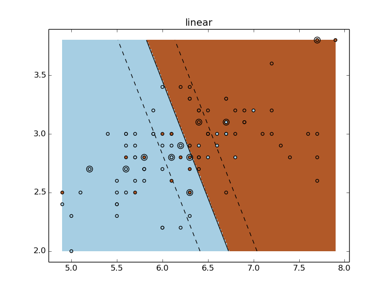
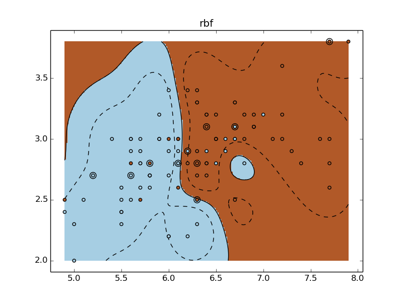
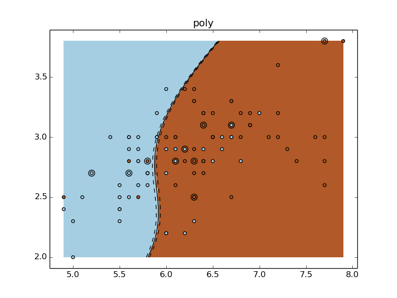
for fig_num, kernel in enumerate(('linear', 'rbf', 'poly')):
clf = svm.SVC(kernel=kernel, gamma=10)
clf.fit(X_train, y_train)
plt.figure(fig_num)
plt.clf()
plt.scatter(X[:, 0], X[:, 1], c=y, zorder=10, cmap=plt.cm.Paired)
# Circle out the test data
plt.scatter(X_test[:, 0], X_test[:, 1], s=80, facecolors='none', zorder=10)
plt.axis('tight')
x_min = X[:, 0].min()
x_max = X[:, 0].max()
y_min = X[:, 1].min()
y_max = X[:, 1].max()
XX, YY = np.mgrid[x_min:x_max:200j, y_min:y_max:200j]
Z = clf.decision_function(np.c_[XX.ravel(), YY.ravel()])
# Put the result into a color plot
Z = Z.reshape(XX.shape)
plt.pcolormesh(XX, YY, Z > 0, cmap=plt.cm.Paired)
plt.contour(XX, YY, Z, colors=['k', 'k', 'k'], linestyles=['--', '-', '--'],
levels=[-.5, 0, .5])
plt.title(kernel)
plt.show()
Total running time of the example: 8.48 seconds ( 0 minutes 8.48 seconds)